Viewer¶

The Inscoper Viewer provides tools for visualizing data acquired with Inscoper I.S.

Open images¶

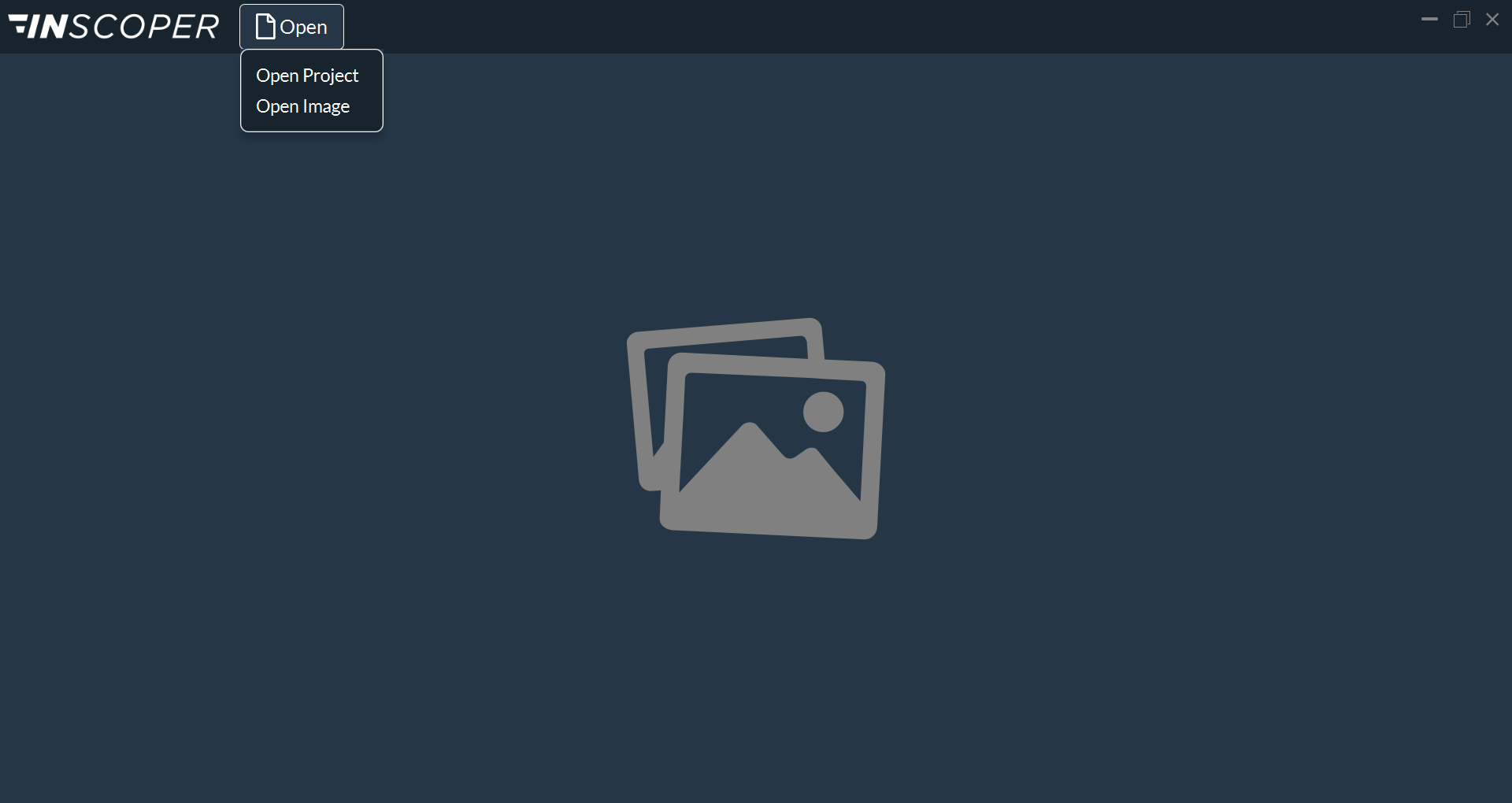
Two ways to open your images:

• Open Project: Select the directory where your project is saved.
• Open Image: Select the directory where your images are saved.

You can open multiple images and find them in the drop-down menu.

Interaction with Images¶

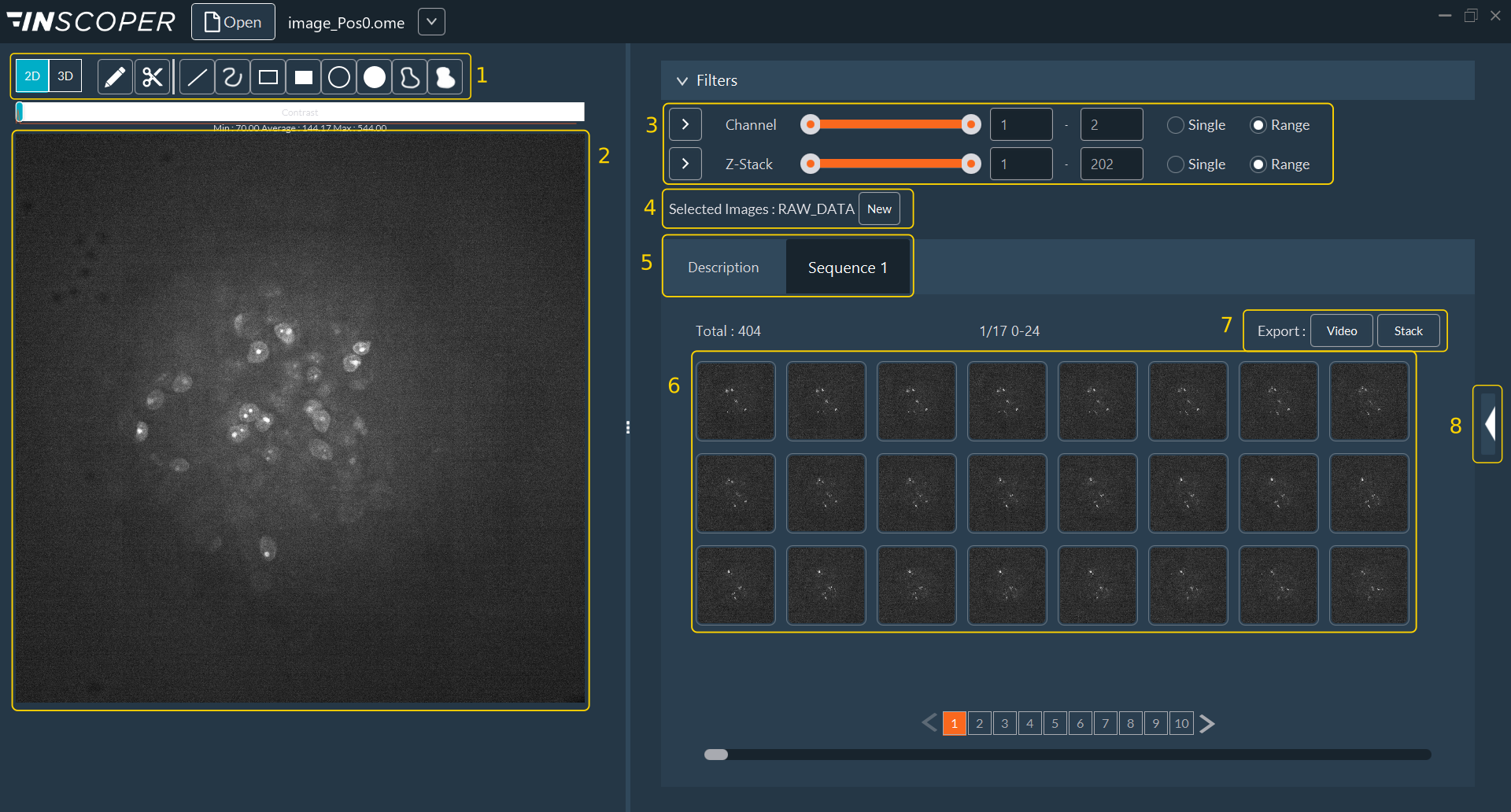
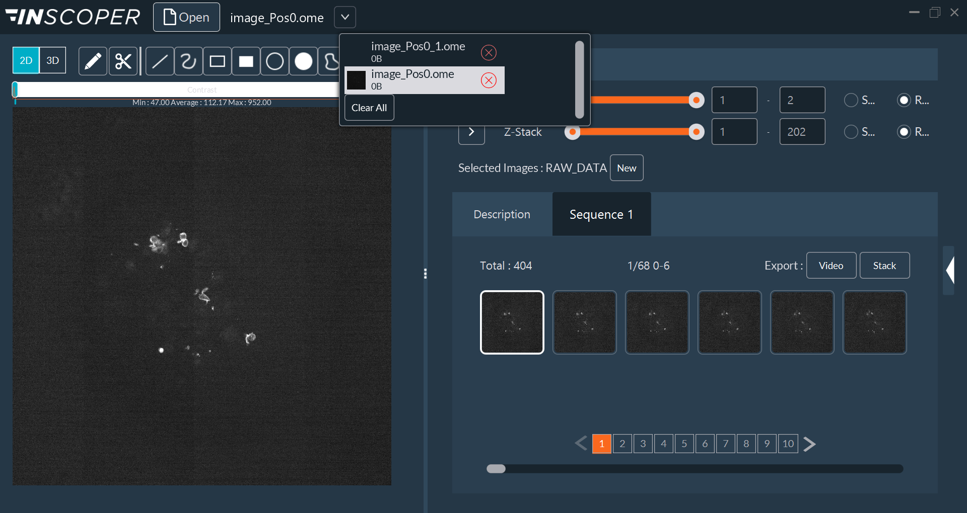
1. ROI tool and 3D Viewer
2. Image Canvas: View images in the viewer.
3. Filters: Use dimension-based filters to search your dataset. Select individual images or full groups. Click the Play button adjacent to a dimension name to animate the sequence.
4. Data Processing: Select output images for post-acquisition processing.
5. Graphics Mode: Switch viewing modes to visualize quantitative data charts.
6. Thumbnail Gallery: Browse miniature representations of all acquired images.
7. Export Options: Save the currently viewed sequence as an MP4 Video or a TIFF Stack.
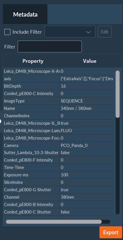
8. Metadata Access: Reveal the hardware and experimental parameters tagged to the images.

3D Viewer¶

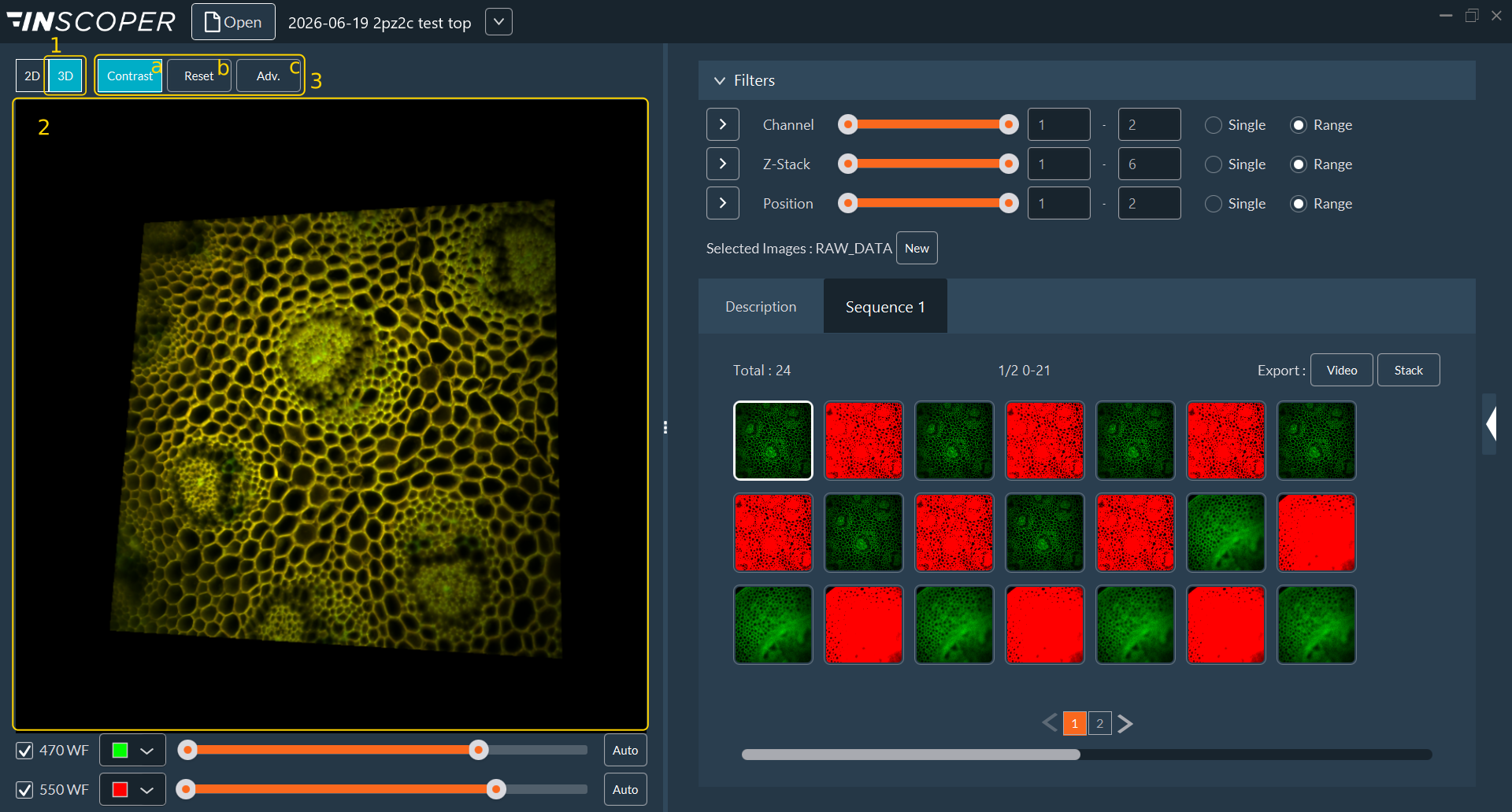
1. Click the 3D button to launch the volumetric viewer.
2. 3D visualization canvas.

3. Adjust rendering options and parameters:

   1. Contrast: Display the LUT and adjust the contrast bar below the 3D view.

   2. Reset: Restore the default 3D camera view.

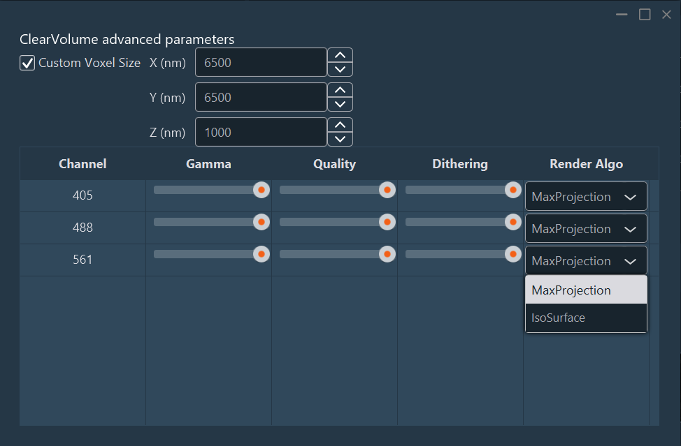
   3. Advanced: Access detailed rendering parameters per channel:

      • Voxel Size (nm).
      • Gamma: Apply a non-linear gamma curve to adjust contrast.
      • Quality: Adjust rendering quality for navigation.
      • Dithering: Reduce banding/aliasing artifacts.

      • Render Algorithms:

        • MaxProjection: Displays only the voxels with the maximum intensity encountered along the viewing ray.
        • IsoSurface: Renders a 3D surface connecting points of equal intensity value.

   

Interacting with Graphics¶

Interact with charts by adjusting their appearance, adding time markers, or exporting raw data. Hover over a graph to access its toolbars.

• Pan: Click and drag the mouse wheel (middle click) to pan across the graph.
• Zoom: Scroll the mouse wheel to zoom in and out. Click and drag to select a region to magnify.
• Jump to Image: Left-click a data point on the graph to view the corresponding image.
• Reset View: Right-click within the graph to restore the default axis scaling.

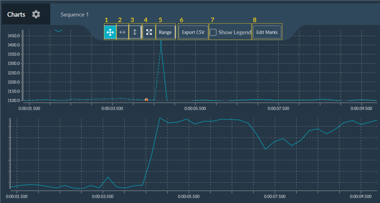
Graph Tools¶

1. Enable the XY zoom mode
2. Enable the X zoom mode
3. Enable the Y zoom mode
4. Reset zoom or enable auto-ranging.
5. Manually override the axis ranges.
6. Export the raw graph data to a .csv file.
7. Toggle curve legends.
8. Add Markers: Annotate the timeline with event markers. Markers can be exported to a .csv file.

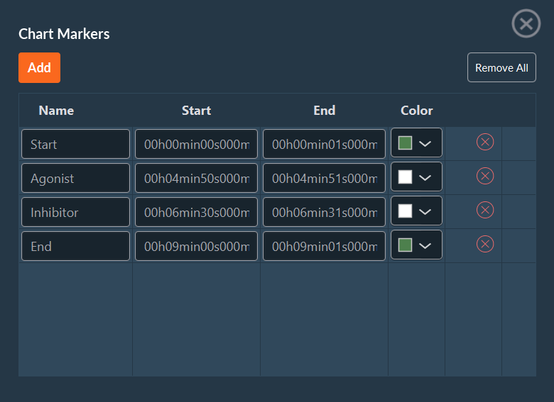
Use this window to add information about your experiment as markers. These fully customizable events can relate to the acquisition itself (start, pause, end), external events (addition of an inhibitor, medium supplementation), or others. Save these markers to a .csv file and reuse them at any time.

Image Processing¶

Apply post-acquisition data processing from the Visualization tab.

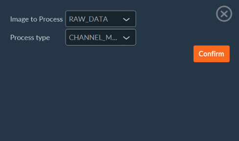
1. Select the target sequence from the image drop-down list.
2. Choose the desired data processor.
3. Click Confirm to execute.

Example: Tiling Stitching¶

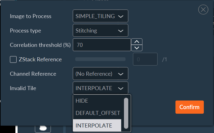
1. Select the image to process.
2. Select the Stitching process type (refer to the stitching algorithm for details on the registration and blending calculations).
3. Set the correlation threshold (%) for image stitching (the minimum correlation score, \(T_{\text{corr}}\)$T_{\text{corr}}$, required to validate the alignment between adjacent tiles; boundaries scoring below this threshold are flagged as invalid, triggering the configured fallback behavior).
4. Optional: Select a Z-stack reference, i.e. the focus plane used to calculate the stitching coordinates.
5. Optional: Select a channel reference, i.e. the channel used to calculate the stitching coordinates.

6. Define the fallback behavior for invalid tiles (uncorrelated):

   • HIDE: Discard the tile from the final image.
   • DEFAULT_OFFSET: Place the tile based solely on its recorded mechanical stage coordinates.
   • INTERPOLATE: Interpolate the tile's position based on the calculated offsets of surrounding valid tiles.

7. Click Confirm.

Data Export¶

Export sequences as MP4 videos or multidimensional TIFF stacks via the Export menu (Toolbar Item 7).

Video Export¶

Use dimension filters to isolate the image sequence, then click Video from the Export drop-down menu.

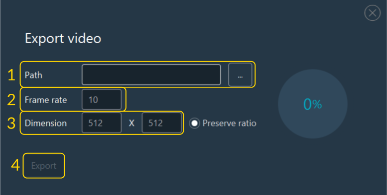
To export a video:

1. Select the destination file path.
2. Verify the sequence to export.
3. Select the video format/codec.
4. Click Export.

Stack Export¶

Use dimension filters to isolate images, then click Stack from the Export drop-down menu to generate a multidimensional TIFF.

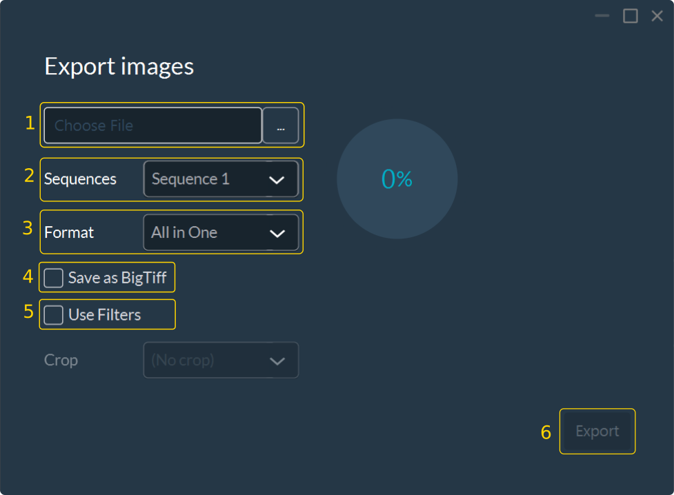
To export a stack:

1. Select the destination file path.
2. Verify the sequence to export.
3. Select the data format.
4. (Optional) Check Save as BigTiff if the expected file size exceeds 4 GB.
5. (Optional) Check Use Filters to apply your visualization filters to the export.
6. Click Export.

Metadata Access¶

A white triangle appears on the right side of the window. Click it to access all metadata, including the camera, light source, and microscope settings. Use the search bar and filters to locate specific parameters. To export the list, click Export at the bottom right of the screen. All metadata are Bio-Formats compatible.