Data Processor
Use the Data Processor to customize data visualization and analysis pipelines during and after image acquisition. View raw image streams, monitor fluorescence intensity graphs, or apply post-processing.
Interface Description

In User Mode, access pre-configured data processing pipelines. Select a pipeline from the drop-down menu and begin the acquisition.
In Expert Mode, click the Switch to Data Processor button to build custom data processing workflows.
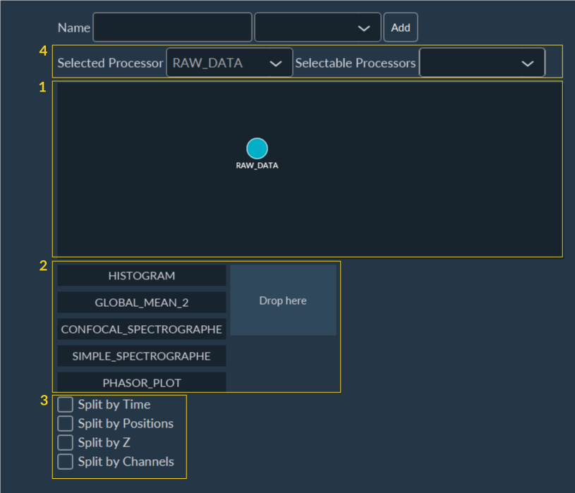
- Workspace: The canvas for creating and routing data processing workflows.
- Visualization Tools: Controls for customizing how data is displayed.
- Dimension Analysis Tools: Tools for analyzing data separated by dimension (e.g., assessing Z-stacks or time-lapses).
-
Image Visualization Customization: Controls for viewing images post-processing:
- Selected Processor: Choose which specific processing node's output to view live during acquisition.
- Selectable Processor: Choose which node outputs will remain available for review in the visualization tab after the acquisition concludes. By default, the system selects all processing steps.
Note
The available processing options depend on the system's specific hardware and license configuration.
Creating a New Data Processing Workflow
-
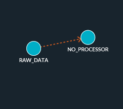
Every workflow originates with the raw images, represented by a root node named RawData. To process these images, create a new node by right-clicking RawData and selecting New Node.

-
The system generates a new, empty node. To assign a processing operation to this node, double-click it, or right-click and select Edit Node.
Tip
For improved readability, right-click the workspace and select Sort Nodes to automatically arrange the pipeline. You can also manually reposition nodes by dragging and dropping them.
-
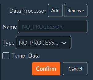
In the node properties window, use the Type drop-down menu to select the desired processing algorithm (e.g., Stitching, Maximum Projection, Background Subtraction).
- Check the Temp. Data box to prevent saving the output of this specific step to disk. This reduces processing overhead and minimizes storage space requirements.
Available Processing Operations
| Processor | Description |
|---|---|
NO_PROCESSOR |
Passes the data through without modifying it. |
SIMPLE_TILING |
Positions each image at its coordinates within a tiling grid. |
STITCH_TILING |
Stitches adjacent images of a tiling acquisition by blending overlap regions. (Note: Requires SIMPLE_TILING to be applied first). |
STANDARD_DEVIATION_ON_FLY |
Calculates pixel intensity standard deviation across an image stack. |
SHADING_CORRECTION |
Corrects uneven illumination and optical artifacts (e.g., sensor dust). |
FILTER |
Reduces noise by removing anomalous pixels (despeckling). |
TIME_MAX |
Performs a maximum intensity projection across the Time dimension. |
FOCUS_MAX |
Performs a maximum intensity projection across the Z-stack dimension. |
TIME_AVERAGE |
Calculates the average pixel intensity across the Time dimension. |
FOCUS_AVERAGE |
Calculates the average pixel intensity across the Z-stack dimension. |
CHANNEL_MULTICOLOR |
Merges images from multiple channels into a multi-color composite. |
SUBTRACT_BACKGROUND |
Subtracts the background signal to improve image contrast. |
CHANNEL_RATIO |
Calculates the ratio of intensities between channels to measure relative changes. |
MULTI_CHANNEL_MERGE |
Merges channels natively (primarily used in SPIM workflows). |
Tip
You can execute all processing steps either during or after acquisition. When run during the acquisition, the processed data updates continuously and saves directly to the final output file.
Customizing Data Visualization
Customize the display of acquired data, such as tracking the evolution of fluorescence intensity over time.
Setting Up the Visualization Window
-
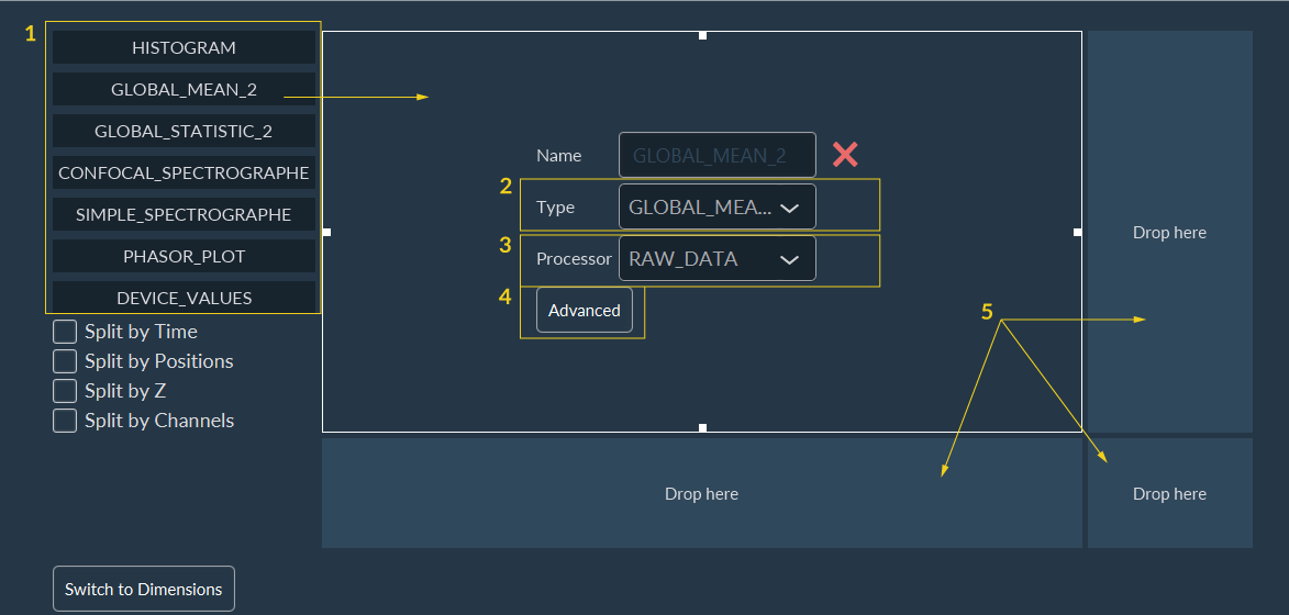
Select the Data Type: Choose what metric to display during the acquisition:
- Histogram: Monitors the evolution of the pixel intensity distribution.
- Global mean: Monitors the average image intensity across an acquisition sequence.
- Global statistic: Similar to Global mean, but includes additional statistical metrics (e.g., variance).
- Device values: Periodically retrieves and plots telemetry from connected hardware devices.
-
Assign to a Panel: Drag and drop the selected data type into a view panel. Change this data type later using the panel's drop-down menu.
- Specify Source: Define the data source (node) for the visualization.
- Customize Graph: Adjust visual graph options, such as axis titles and curve labels.
- Add Graphs: To display multiple graphs simultaneously, drag and drop additional data types into empty view panels.
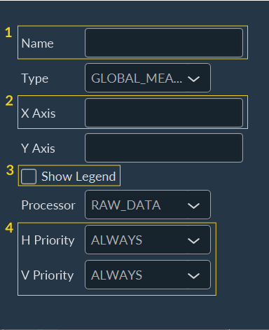
Graph Customization Options
- Set a custom title for the graph.
- Label the X and Y axes.
- Toggle the visibility of curve legends.
- Enable the Always option to ensure the graph remains visible throughout the experiment.
Note
Visualization customization is optional. It aids in data interpretation during acquisition and does not affect the saved acquisition data.